I’d like to talk to you about one interesting thing. Everyone “works” with it daily without realising it. We will talk about the land relief or terrain.
According to official definition terrain is a “the vertical and horizontal dimension of land surface”. So, it is only a shape. But this is the case when it’s safe to say that, for an average person, the shape is more important than the contents. Imagine an iron ball and a plastic one. What do they have in common? They move around easily due to the form they have. Push it and it rolls.
Terrain also gives certain features to natural and man-made objects depending on their location. For instance, in our hemisphere the south facing slopes or building walls will always get more sun light than others. That is why the southern slopes of a hill will host specific biocenoses, soil variations are formed. Moreover, the lithological structure of this hill will play a secondary part in landscape formation.
No natural or anthropogenic process takes place without some influence of the terrain. Water flowing in a river, wind direction, urban development planning, switching gears when going uphill… We have to accept the terrain, live with it, use it’s features to suit our purposes.
However, it’s good to learn as much as possible about something we are using. And in this case the use efficiency will be directly proportional to the amount of knowledge we have.
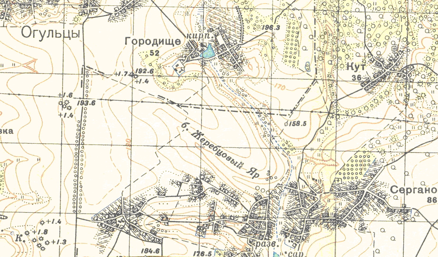
Where do we get information about the terrain? There are plenty of sources and ways at the moment. The most mundane way is using physical or topographic maps. As the features of terrain are shown in contour lines – curves with equal altitude at each point.
Figure 1. Traditional way of presenting land relief going far back to school textbooks
Years of experience of working with paper maps have formed a deep methodology for making morphometric calculations. From simple slope calculations to a more advanced thickness of the horizontal partition mapping. Surely, with technological advancements traditional terrain representation is gradually changed by other more practical methods. I’m sure, most of our readers have seen 3D digital models of separate land forms as well as larger areas.
These visual replicas of natural features are created based on digital elevation models (DEMs). A DEM is “a digital model or 3D representation of a terrain’s surface created from terrain elevation data.” The models are based on altitude or bathymetry points serving as nodes on an irregular triangular network of a regular grid, or isolines.
Simply put, a DEM is a computer model that contains detailed information about altitude. Furthermore, there is a differentiation between a digital elevation model (DEM), digital terrain model (DTM) and digital surface model (DSM). Where a DTM represents a set of morphometric parameters’ derivatives.
Initial digital data on terrain features may he represented in two commonly used ways. These are a regular and an irregular ways of presenting data: a grid and a triangulated network. The first is supported by the famous “monster” – ESRI, and is commonly known as GRID-model. The second is called TIN (triangulated irregular network).
GRID-model has a raster structure that is created by splitting space into finite cells or pixels. These are normally square features containing information about altitude above sea level. As a rule GRID is a basis for global and local altitude models. In fact, United States Geological Service (USGS) as part of the National Map project offers five terrain data sets. These differ by the production technology, resolution and extent. GRID model is also the basis of open global DEMs, like GMTED2010 and ASTER GDEM2.
TIN structure is well described by its name. It is based on a set of irregularly placed nodes that are connected by edges forming triangles. A polyhedral land relief model is formed, it consists of numerous triangles with altitude points and the nodes.
 |
 |
| TIN | GRID |
Figure 2. Two ways of terrain representation
Each of these models has advantages and disadvantages. Usually, a TIN uses several times less storage space that a GRID, as it has a vector structure. It also requires more processing time due to the same fact. It is considered that TIN is better suited to represent mountainous regions, whereas GRID is better for flap terrain.
Moving on, we’ll talk a bit about the theory.
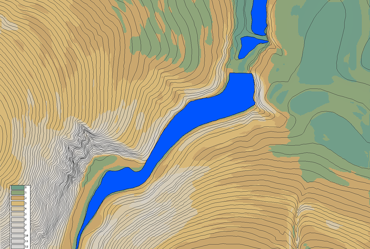
For instance, in a GRID model visual analysis of the surface that is created by altitude cells is quite straight forward. It appears that even a high school student can figure out the image, and see at least the hills and hollows (We surely hope so!). Analysing a 3D visualisation (figure 3) of a surface is even more simple, that is too obvious.
 |
 |
Figure 3. 3D terrain visualisation
This model, however beautiful it may be, is not too practical. As the serious work requires serious maths and some terrain assessment criteria.
If you’d like to have a look at the area depicted by our elevation surface check it out on the map or even drive there, some 13 km from Kharkiv along the Kyiv highway.
Undoubtedly, one of the most fundamental and widely used geomorphic parameters are slope and exposition of the surface. Let’s start with slope, which is a measure of surface steepness, and is calculated “by finding the ratio of the ‘vertical change’ (a) to the ‘horizontal change’ (b) between two distinct points on a line” (figure 4).
Figure 4. Slope steepness
So, the slope value corresponds to tan(α). Speaking more mathematically, the slope is the first derivative of the height, because it describes the intensity of its value changes of in space.
Nearly any GIS software is capable of turning a raster model into a slope map (in case of GRID) or to determine the steepness of edges/triangles (in case of TIN).
Lets have a look at working with the raster model. Here, a Zevenbergen-Thorne (1987) algorithm is generally used.
Here are its main stages having a 3×3 submatrix as an example (figure XXX). All the calculations aer made for the central cell highlighted in blue. Numbers in the cells represent altitude (z), L – is the distance between the cell centres, in other words – raster resolution. The pixels influencing our calculations are highlighted in yellow.
First, the altitude change gradients along two main axes, x and y, are calculated:
dz/dx = [ 62 – 61 ] / 2*L
dz/dy = [ 65 – 59 ] / 2*L
Next, ‘integral’ slope is calculated for the central cell:
slope = arctg (√ ([dz/dx]2+ [dz/dy]2))
Figure 5. Slope calculation
Next, all that is left is running this algorithm for the whole raster. As a result all the altitude values for each pixel of the DEM will be recalculated into slope values. A slope steepness map is made (figure 6).
Figure 6. Slope steepness map
That’s great, but what is the use for all of these maths and GIS stuff for an average person?
True, let’s get back to land, but in the next post.
__________________
Grapics by Chris Cole from Noun Project is used in this post

