We have already posted a material about supervised classification algorithms, it was dedicated to parallelepiped algorithm. Now we are going to look at another popular one – minimum distance. In contrast with the parallelepiped classification, it is used when the class brightness values overlap in the spectral feature space (more details about choosing the right classification type here).
Theory
First, we will learn about the theoretical background of the minimum distance classification using a simplified example. The simplest case is the 2-dimensional spectral feature space. You can see it in figure 1. The axes correspond to the image spectral bands. Each pixel of the satellite image corresponds to a point in the feature space. The figure shows three classes, that are in red, green and blue points. The red point cloud overlaps with the green and blue ones. There is also a black point cloud that does not belong to any class. After the image is classified these points will correspond to classified pixels.

Fig. 1. An imaginary example of a minimum distance algorithm to be used to distinguish classes
Figure 1 on the left shows a situation where the classification does not include the possibility of unclassified pixels. And Figure 1 on the right, on the contrary, a case with unclassified pixels in the results of the classification. The grey arrows show the distance from the green point A and the red point B to the centers of green and red classes. We see that both points are closer to the green class center. Therefore points A and B will be classified by the minimum distance to the green class. Here we see the principle of determining membership in the class and the source of errors in the classification. But the number of errors will be less than when we limit the classes to rectangles, as in the classification by the parallelepiped algorithm. That is why when brightness values of classes overlap it is recommended to use a minimum distance algorithm, rather than a parallelogram algorithm.
If we assume the presence of unclassified pixels, the algorithm of the minimum distance gets slightly more complicated. Figure 1 shows a black point marked as C. The closest class center to it is the center of the red class. To exclude this point from classification procedure, you need to limit the search range around the class centers. For this, set the maximum permissible distance from the center of the class. Figure 1 on the right shows an example of this. Maximum distances from the centers of the class that limit the search radius are marked with dashed circles. Without this restriction, most black points would be assigned to the red class, and some – to green (fig. 1, left). And with the restriction (Fig. 1, on the right) they will remain unclassified.
You can apply a search restriction of the same value to all classes. This is the case when all classes have a similar spread of values. And if the classes have a very different spread of values, then it is necessary to set for each class its own size of the search radius. This more complex case is shown in Figures 1 on the right when a greater distance from the center of the class is defined for the red class than for the blue or the green one.
Practice
For a practical implementation of the minimum distance algorithm in ENVI, we will look at an example of classifying woody vegetation and reservoirs on a satellite image. A snippet of this image is shown in Figures 2 on the left. It was taken from the US satellite Terra on September 16th, 2015, with ASTER VNIR equipment. It covers the floodplain of the Siversky Donets River on the borders of the Zmeivsky and Balakliya districts of the Kharkiv region, between the villages of Cherkassy Byshkin and Nizhniy Byshkin in the west and the town of Andriivka in the east.
In the image, three classes need to be distinguished: water surfaces, coniferous and deciduous forests. Among the water bodies, there is Siversky Donets river, numerous oxbows on the floodplain and Lake Lyman. The deciduous forests are represented mainly by small-scale floodplain forests on the left bank of the Donets and the broad-leaved tract of Tyundik on the right bank. Coniferous forests are Andreevsky Birch, which grows on the left-bank terrain of the Donets, between its floodplain and Lake Lyman.
ASTER VNIR image has three channels with the spatial resolution of 15 m/pixel.The bands cover the green, red and infrared parts of the spectrum. Figure 2 shows a false color composite of the 3-2-1 band combination (infrared – red – green). This composite shows the conifers as brown, the deciduous trees as bright red. The water bodies appear as black or dark blue.
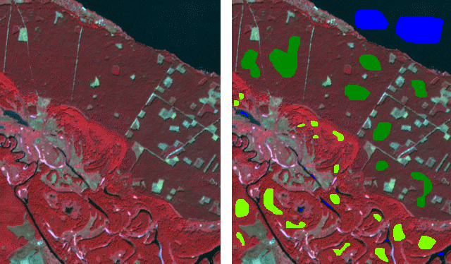
Fig. 2. ASTER image snippet (left) and ROIs (right)
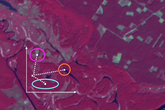
The training regions of interest for our three classes are shown in figure 2. When analyzing the posilions of the ROI pixels in the n-D feature space, we see that they overlap (fig. 3). That is why this case we should use the minimum distance algorithm for our classification.
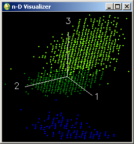
Fig. 3. Training regions in the 3-dimensional spectral feature space
So, we have made sure that minimum distance is the right algorithm. Next, we will go through the process step by step.
1) To start the classification process in Toolbox choose Classification→Supervised Classification→Minimum Distance Classification (fig. 4). Classification Input File window appears. Select the image that needs to be classified.
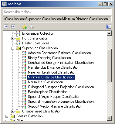
Fig. 4. Minimum distance algorithm in the ENVI toolbox
2) After selecting an image Minimum Distance Parameters window will appear (fig. 5). The settings window for the minimum distance algorithm classification has a similar interface to the one for parallelepiped algorithm. It also has four blocks:
- list of ROIs (Select Classes from Regions)
- classification parameters (Set Max stdev from Mean and Set max Distance Error)
- settings for saving the output (Output Result to).
- Setting for saving rule images (Output Rule Images?)
The only difference is the parameter that sets the boundaries of the classes. More precisely, in the minimum distance algorithm, there are two such parameters: maximum standard deviation from the mean (Set max stdev from Mean) and maximum distance (Set max Distance Error). You can set one of the two options and leave the second one blank. Or you can configure both options. In this case, the program will use the parameter that restricts the search for pixels around the class center more.
If we choose not to have unclassified pixels, then the radio button needs to be set to None. Otherwise, set the radio button to Single Value or Multiple Value.
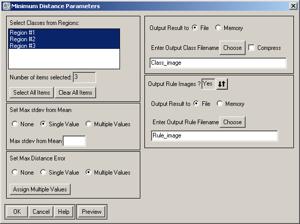
Fig. 5. Minimum distance settings window
The Single Value option sets the same classification parameter for all classes. Figure 5 shows that this option is selected for the Set max stdev from Mean parameter. To set a separate value for each class, select Multiple Value (it is selected for Set max Distance Error in figure 5). Next, press the Assign Multiple Values button. A window will appear where parameters for each class need to be assigned (fig. 6).
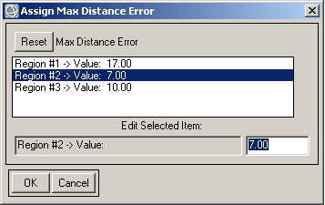
Fig. 6. Setting up the parameter values for each class
3) After the classification parameters were set, ROIs need to be selected in Select Classes from Regions. Then, set the output saving options (classification map and rule images).
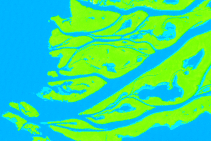
4) The last image shows the result – classification map.
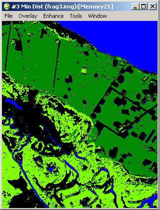
Fig. 7. Classification results
It does have small errors, but the map can be improved by classification post-processing. We will look at it in more detail in one of our future posts.


