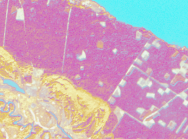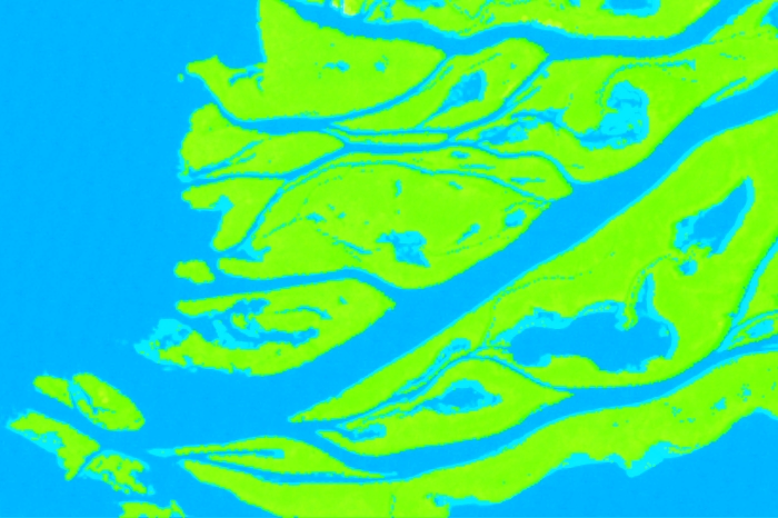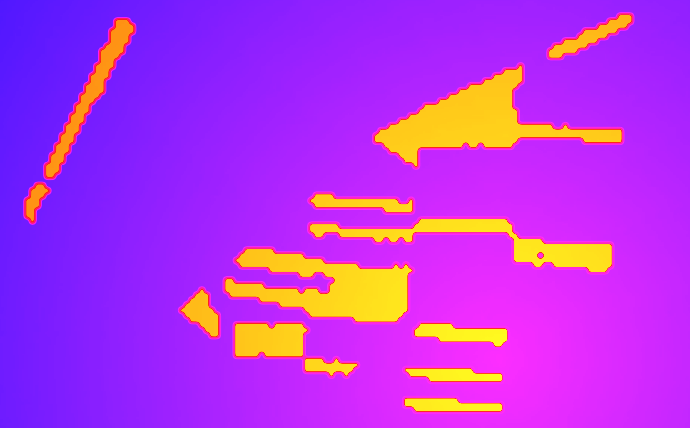
The main result of supervised satellite image classification process is the classification map. But apart from it, you can still get another result – the rule image. In this post, we will look at what it is.
When we perform supervised image classification, the software calculates a mathematical criterion (which depends on the classification algorithm) for each pixel. The value of this criterion defines the class the pixel belongs to. For the algorithm to be able to calculate the criterion, reference classes must be specified. This is done by the user. To allow the program to split classes by criterion, you must specify the threshold value of this criterion. This is also done by the user. And then the algorithm is doing everything on its own, without user intervention. As the classification output, the user receives a completed classification map. This map indicates each pixel of the image belonging to a specific class. Usually, this is exactly what the user is interested in.
However, sometimes it is not only what classes the pixels belong to that needs to be determined. The user may also want to see the criterion values for image pixels that were used to distinguish the classes. In other words, the user may be interested in knowing to what extent does a pixel match the class reference.
How can it be done, when the classification process itself is hidden from the user? To do this, you can create a so-called rule image during the classification. This is a multi-layered raster image. It has the same number of layers as the classes in the classification. The value of each pixel in a separate layer is the value of the mathematical criterion by which the program determined whether the pixel belongs to a class or not.
In this post, we will look at what visualization tools for image rules exist in ENVI, and how to view the quantitative values in these images. We illustrate this by an already familiar example of decoding from a previous post about the minimum distance algorithm. Why take this example? Because the mathematical criterion for the minimum distance algorithm is the Euclidean distance between the center of the class and the pixel, this is the most intuitive mathematical criterion. Because this is the usual distance with which we are all familiar with.
Creating and visualizing rule images
To create a rule image, we need to do the following.
The first step is to create training areas using ROIs.
Next step is to run supervised classification from ENVI Toolbox. In the settings section of the classification options, there is the “Output Rule Images?” option that creates a rule image (Figure 1). Once you have configured everything else, you need to use the arrow buttons to set this parameter to Yes (Figure 1). And then select a way to save the image (Enter Output Rule Filename). It can either be stored in a temporary memory (Memory), or stored in a file (File).
There are three ways to visualize image rules in ENVI:
display a separate layer (rules for a separate class) in shades of grey,
display a separate layer (rules for a separate class) as a pseudo-color image;
synthesis of two or three layers (rules for two or three classes) as a color image (RGB-composite).

Fig. 1. Rule image creation option (marked with a red border) in the settings window of the minimum distance algorithm classification
By default, the rule images in ENVI are displayed as RGB-composites. R, G and B layers of the composite correspond to the first, second, and third layer of the rule image. An example is shown in Figure 2. In the center there are rules for the image in the RGB-combination 1-2-3 (water – coniferous forests – deciduous forests). For comparison, on the left in Figure 2, a classification map is given, in which the blue marks water bodies, green – coniferous forests, light green – deciduous forests.

Fig. 2. Classification map (left), rule image in the combination 1-2-3 (center), rule image in combination 3-1-2 (to the right)
If necessary, you can change the order of the image rules in the RGB composite. To do this, you need to right-click on the layer name in the Layer Manager. A popup menu appears. Choose Change RGB Bands … (Figure 3). After that, the Change Bands window will appear (fig. 4).

Fig. 3. Start the procedure for changing the layer order in the RGB composite
In the Change Bands window beside the name of each layer (left), there is a colorless square. Click on these squares with the left mouse button. The first click sets the R component of the RGB composite, the second sets the G component, the third sets the B component. When executing these actions, the squares get the appropriate color. When all is specified, you need to click the OK button in the Change Bands window (Figure 4).

Fig. 4. Change the layer order in the RGB-composite
The result of changing the band combination of RGB composite is shown in Figure 2 on the right. The similar images (Fig. 2, center and right) have a spectacular look, but they are difficult to interpret. It is easier to interpret a separate classification rule image. To display it in shades of grey, in ENVI menu select the command File → Data manager. The Data Manager window (Figure 5) appears.
![]() It can also be opened by pressing the F4 button on the keyboard or by pressing the button in the ENVI toolbar. In the data management window, select one of the layers of the rule image and click the Load Grayscale button.
It can also be opened by pressing the F4 button on the keyboard or by pressing the button in the ENVI toolbar. In the data management window, select one of the layers of the rule image and click the Load Grayscale button.

Fig. 5. Data manager window
An example of displaying a single raster layer in grayscale is shown in Figure 6. This is a rule image of the minimum distance classification for coniferous forests. The image tone indicates the value of the classification criterion. The darker the shade of a grey color, the smaller the value of the criterion. In the example given, the criterion is the distance from the center of the class of coniferous forests. The darkest part (almost black) of the image in Figure 6 corresponds to the coniferous forest. The dark grey color is mostly deciduous forests, the pixels have a distance to the center of the class of coniferous forests more than the pixels that truly belong to that class. And the most distant from the center of this class is the water and some clear cuts in the forest, having respectively a light grey and almost white color.

Fig. 6. The minimum distance classification rule image for coniferous forests
To distinguish the difference between objects in the rule image for a particular class, you can change the black and white range to another one. To do this, in the Layer Manager right-click on the layer name. Choose Change Color Table → More … from the context menu. The Change Color Table window appears. In this window, you can choose from many palettes or create your own (Figure 7).

Fig. 7. Choosing a color table and an image of the classification rule for water class shown in this table
View quantitative values of a single pixel
There are three ways to view the individual pixel values in ENVI:
– pointer values,
– spectral profile,
– spatial profile.
The first method is exclusively quantitative. And the second and third ones are quantitative and graphic methods.
![]() You can also click on the button in the panel. A Cursor Value window appears, it displays the values below the cursor (Figure 8). When we move the mouse pointer over a pixel, this window shows its value as well as geographic coordinates. You can also add a crosshair sight to make it easier to capture the position of the pixel, the value of which we are viewing.
You can also click on the button in the panel. A Cursor Value window appears, it displays the values below the cursor (Figure 8). When we move the mouse pointer over a pixel, this window shows its value as well as geographic coordinates. You can also add a crosshair sight to make it easier to capture the position of the pixel, the value of which we are viewing.
![]() Press the crosshair button in the ENVI panel bar.
Press the crosshair button in the ENVI panel bar.

Fig. 8. Cursor value display
In the Cursor Value window, we can read several parameters (from top to bottom):
– Geo: geographic coordinates of the pixel in degrees,
– Map: rectangular coordinates of the pixel in meters,
– MGRS: pixel coordinates in the MGRS (Military Grid Reference System),
– Proj: cartographic projection of the image,
– file name
– File: display pixel coordinates,
– Data: pixel value.
If the image is multilayered, then in the Data parameter will display the pixel values of each layer in square brackets, separated by a comma. The value order will match the layer order in the image from first to last. In our example, we have the following order of layers in the image of the rules: water, coniferous forests, deciduous forests. Knowing this, we can draw from Figure 8 that the pixel on which the cursor was placed is likely to belong to the class of water. Because the pixel lies closest to the center of this class, the shortest distance in the multidimensional spectral feature space. We can also say that the largest distance to the center of the class is for deciduous forests. This distance is approximately 1.5 times more than the distance to the center of the class of coniferous forests, and approximately 50 times more than to water.
2) A spectral profile is a graph that displays how the values change in a separate pixel of a raster image from a layer to a layer.
![]() To create one, click the Spectral Profile button on the ENVI toolbar or type Alt + Z from the keyboard. To add multiple profiles to the graph, you should left-click on the pixels while simultaneously holding Shift on the keyboard.
To create one, click the Spectral Profile button on the ENVI toolbar or type Alt + Z from the keyboard. To add multiple profiles to the graph, you should left-click on the pixels while simultaneously holding Shift on the keyboard.
Figure 9 on the left is a rule image. There are three dots on it. The blue dot is on the water surface, the dark green dot is located in the pine forest, and the light green one in the deciduous forest. The Spectral Profile window is shown to the right of this figure. It contains spectral profiles for these three dots. This is the same information as in the Cursor Value window in the Data item (Figure 8). But it is shown graphically.
The spectral profile also allows you to set precise values. To do this, you must click the left mouse button along the curve. In the lower left corner of the Spectral Profile window, pairs of values X and Y will be displayed. Y is the value of the mathematical classification criterion that represents the rule image. X is the layer number in the rule image. The color of the values of X and Y indicates which curve they belong to. So, in Figures 9 there is a value that shows how much the point in a coniferous forest is far from the reference of coniferous forests.

Fig. 9. Spectral profiles of the rule image (right) and the points for which they were created (left)
3) The spatial profile allows you to see how values change in a separate layer of rule images along a user-defined line (transect). To create a profile, click the Arbitrary Profile (Transect) button. Left-click on the image to lay out the transect (in Figure 10 it is marked with a dashed line). Then, right-click and select Complete and Accept Polyline from the context menu to complete the transect.

Fig. 10. The spatial profile of the classification rule values (right) along the user-defined transect (left)
The transect marked on the left in Figure 10 was laid from the north to the south. And in the Arbitrary Profile window (fig. 10, on the right), the direction of the spatial profiles is from the left to the right in this direction. Analyzing these profiles, we see two facts. The first is a sudden change in the values in two places, indicating the boundaries of classes (first between water and coniferous forests, then between coniferous and deciduous forests). The second is the variation in the nature of the course of profiles within the classes. In the water class, the fluctuations of the profiles are small, in coniferous and deciduous forests – on the contrary, quite large. The greater the fluctuation within the class, the more heterogeneous its surface in the area.
So, we figured out what sort of classification rules were, how to create them, how to visualize them, and how to view the quantitative values of the pixels of these images. By reading this post, you could reach one interesting point. And can it not be possible to distinguish classes directly based on the analysis of rule images? This is really possible. This will be the topic of the next part on rule images: classification based on rule images.


