When we perform image classification, we try to get the best possible result. Despite this, often the result of the classification, although good, is not perfect. And no classification procedure settings can improve the accuracy of class recognition. In this case, it is possible to improve the result using post-processing algorithms. They include procedures for combining classes, smoothing the boundaries of classified areas, combining small areas, isolating small areas. These procedures are used in various combinations and sequences, specific to the task of classification.
In the broad sense, post-processing also includes an assessment of the accuracy of the classification: creating an error matrix and ROC curves. We will not look at those processes in the current post.
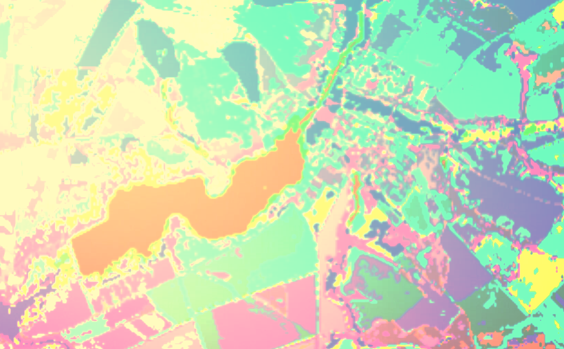
We will try out post-processing using the following example. A fragment of a Landsat-5TM satellite image (Fig. 1, right) was classified using the k-means algorithm. This fragment covers the territory around the Murom Reservoir, located at Murom River in the Kharkiv region.

Fig. 1. Landsat-5TM image, band combination 7: 5: 3 (left) and classification map (right)
The classification map is shown in Figures 1 to the left. 12 classes were distinguished. It is necessary to transform the classification map so that it has only two classes – the water surface and other surfaces. In addition, it is necessary that the water surface class contains only the reservoir. And small lakes should be taken away. We have used the result of this classification in the post about the automated change detection. Now we will analyze how data from that post was prepared.
Class identification
On the map of classification, we see only the colors of classes. We do not know numbers corresponding to classes and the relation between classes and objects in the field. This is what is first defined before the post-grading processing. Here we are talking about the case of unsupervised classification. When we do a supervised classification, of course, we know what classes correspond to what objects.
To identify the classes, you must drag the classification map up in the table of contents to show it above the satellite image (Fig. 2). Then you can expand the list of classes. Then you need to remove the check boxes for all classes and check them one at a time. Separate classes will be depicted on top of the image so that you can see the objects below and around them.
Figure 2 on the left shows the display for classes that correspond to the water surface. They are class number 1 (red) and class number 2 (green). The second class corresponds to deep water and green to shallow water. As we see, there are many errors in the green class. It mistakenly contains some areas in the Murom River valley. Also among the errors are some pixels that actually belong to forests. Next, we will eliminate these errors by means of sieving.

Fig. 2. Classes overlaid on top of the satellite image
If there is an excessive number of classes, then they must be joined together. This is exactly our case here. Unsupervised classification will often result in more classes than are necessary for the final result.
1) To start the process, select Classification→Post Classification→Combine Classes in the Toolbox. After that, you will have a window in which you need to select a classification map.
2) After selecting the classification map, a Combine Classes Parameters window will appear (Fig. 3, left). At the top of this window, there are two lists – the classes we select (Select Input Class) and the classes that we associate the pixels to (Select Output Class). To select a pair of classes to merge, specify one class in the left-hand list, and another class in the right-hand list. After that, click the Add Combination button. A pair of classes will be placed to the Combine Classes Parameters list located at the bottom of the Combine Classes Parameters window. When you have paired all classes, click OK. In our example, we combine the first and third classes that correspond to the water surface. And all other classes will be set to unclassified pixels.
3) After the pairs of classes are matched, the Combine Classes Output window will appear. In it, the Output Result to switch specifies a way to save results. They can be stored in temporary memory (check Memory) or in a permanent file (check File).

Fig. 3. Selecting classes to merge (left) and empty classes setting (right)
4) In addition, in the Combine Classes Output window, you can specify whether to remove blank classes or not. To do this, use the arrow buttons to set the Remove Empty Classes option to Yes or No. If No is selected the properties of the merged classification map will include all the classes that existed originally. In our example, they would be 12 classes and unclassified pixels. This is not very convenient. It is better to choose Yes so that the properties of the new classification map only contain those classes that actually exist. In our example, this will be one class (water surfaces) and unclassified pixels. This result of class association is shown in Figure 4. Note how many classes are in the classification map and how many of them are indicated in the table of contents.

Fig. 4. Merged classes
Sieving
After combining classes, the next step of post-processing in our example is searching for small areas. This will help to remove both small lakes and errors in the form of small groups of pixels from the classification.
1) To start filtering the pixels of the classification image, select Classification→Post Classification→Sieve Classes in the Toolbox. After that, a window will appear in which you need to select a classification map for sieving. We have the result of combining the classes that was obtained in the previous step.
2) After the data is selected, a Sieve parameters window will appear in which you need to adjust the parameters (Figure 5). Choose the classes for it to be used for sieving (you can choose either all classes or several separate classes). We only have one class, but we need to select it anyway.

Fig. 5. Sieve parameters window
3) Specify the size threshold in pixels in Group Min Threshold. All areas that are smaller than this value will be filtered out. The pixels will be assigned to the Unclassified class. In our example, the threshold of sieving is set to 200 pixels (Figure 5). It will allow you to remove everything except the reservoir from the class of water surface.
4) The “Number of neighbors” option affects the way of determining if a pixel belongs to a group. Select the method using the arrow buttons. There are two options: 8 neighbors and 4 neighbors. 8 of the neighbors means that the pixels in one class belong to one group if they have common sides or corners. That is, if this pixel belongs to a group, then it can have a maximum of eight directly adjacent pixel neighbors because the pixel has four sides and four corners. The option of 4 neighbors means that pixels of the same class belong to one group only if they have common sides. That is, if this pixel belongs to a group, then it can have a maximum of four directly adjacent pixel neighbors.
5) Last configuration – a way to save results (in temporary memory or in a file). The result of the sieving for our example is shown in Figures 6. These data were used to illustrate the previous post.

Fig. 6. Small areas were sieved
In some cases, it is necessary for each class to set its threshold of sieving. But in ENVI this setting is not available. But this problem can be solved. You can repeat the procedure several times so that the result of the previous operation is the input for the next operation. At the same time, each sieving is made for only one class with an individual threshold. Accordingly, the maximum number of sieving operations may be equal to the number of classes.
Clumping
1) Small areas that are located near each other can be aggregated and their boundaries smoothed. To run this post-processing procedure, you must select the Classification→Post Classification→Clump Classes command in the Toolbox. After that, you will have a window in which you need to select a classification map.
2) After choosing the classification map, the Clump Parameters setting window (Figure 7) will appear. First of all, it is necessary to choose the classes for which the aggregation is performed. In our example, there is only one class, but it still needs to be selected.

Fig. 7. Clump parameters window
3) Next adjust the degree of clumping. It affects the size of the sliding window, which searches for neighboring pixels during aggregation. This size is indicated by the Operator Size Rows and Cols: in pixels. The larger this size, the higher the degree of clumping. In our example, the size is 5 by 5 pixels.
4) Last configuration – a way to save results (in temporary memory or to a file). The result of aggregation for our example is shown in Figure 8. You can compare it with Figure 6. The biggest difference seems to be in the southern shore of the reservoir near the dam.

Fig. 8. Clumping results
Majority/Minority analysis
Majority analysis and minority analysis is another way of generalizing a classification map. A neighborhood is formed around a pixel that is defined by distance set by the user. Within this neighborhood, the number of pixels belonging to different classes is counted. If the majority analysis is performed, then the central pixel is assigned to the class that corresponds to most of the pixels in the neighborhood. When analyzing a minority, on the contrary, the central pixel is assigned to a class with a minority of pixels in the neighborhood.
1) To start the majority/minority analysis, you need to select the Classification→Post Classification→Majority/Minority Analysis command in Toolbox. After that, you will get a window in which you need to select a classification map. In our example, this is a classification map that is obtained after the sieving procedure.
2) After choosing the classification map, a settings window for the majority/minority analysis will appear. First, select the classes for which the analysis is performed from the Select Classes list.
3) Using the Analysis method switch, select the type of analysis – Majority or Minority.
4) Then set the size of the analysis window (Kernel Size parameter). If we perform a majority analysis, then we need to add a Center Pixel Weight. It shows how many times the central pixel is counted when determining the distribution of pixels by class (default is 1).
5) Last configuration – saving results (in temporary memory or in a file).

Fig. 9. Majority/minority analysis settings
The result of the analysis of the majority and the minority for our example is shown in Figure 10. The majority analysis was performed for a class of reservoirs and a class of unclassified pixels with the size of the 5-pixel kernel. This procedure has led to smoothing the boundaries. Minority analysis was performed only for the water reservoir class with a 5-pixel kernel. This procedure has reduced the size of the object.


