In a previous post on the topic of spatial statistics, we have shown how to define the type of spatial distribution of discrete objects. But, besides distribution of the objects themselves, a spatial distribution of their characteristics may have a certain interest, as well. For the same objects, some characteristics may feature a uniform type of spatial distribution, and others – aggregated or random (chaotic) type. To define this, the Moran’s I coefficient (‘I’ is the letter, not the Roman digit 1!) can be applied.
Theory
The criterion had been proposed by an Australian statistician Patrick Alfred Pearce Moran (a.k.a. Pat Moran) in the late 1940s when he had been working as a Senior Researcher at the Oxford University. The first publication where the Moran’s coefficient was introduced is dated by 1950 and printed in the British peer-reviewed scientific journal ‘Biometrika’.
First we proceed with some terminology, in fact, we will look solely into “spatial autocorrelation”. Let us begin with a “common” correlation.
Correlation, or correlative relationship, is a kind of relationship between two (or multiple) variables where changes in one variable are accompanied by changes in other variables. Autocorrelation is the same kind of relationship but of one variable with itself. This can happen when measurements are distributed in time or in space. In this case, a relationship may exist between measurements made with different intervals in time or in space. In the first case, the relationship is a temporal autocorrelation, in the second case – a spatial autocorrelation.
The Moran’s I criterion is a coefficient of spatial autocorrelation. Like a “common” coefficient of correlation, it ranges from -1 to +1. How is it related to the character of the spatial distribution of variables? All possible types of variable distribution in space may come to the three modes (fig. 1):
- random (chaotic),
- uniform (even, dispersed), or
- grouped (clustered, aggregated) distribution.
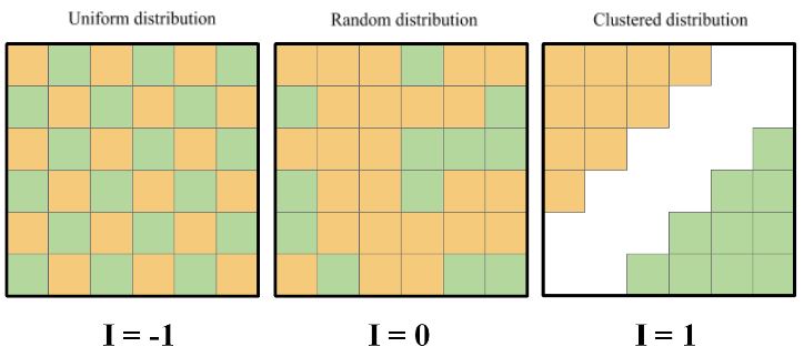
Fig. 1. Types of the spatial distribution of variables
The criterion’s value expected for a random distribution of variables approximates 0. In the majority of cases, its difference from zero is so small that it can be correct to tell that at random distribution of variables the Moran’s I criterion equals zero.
When the Moran’s I criterion approximates 0, a spatial autocorrelation is absent, and values are randomly distributed in space. If the criterion is significantly greater than zero the positive spatial autocorrelation exists, and values are distributed in space with a clustered mode. In the case when the Moran’s I criterion is significantly less than zero the negative spatial autocorrelation exists, and values are distributed in space uniformly.
Now we proceed with calculations of the Moran’s I criterion. This is quite a simple but time-consuming procedure, especially when the number of objects is high. However, modern software allows doing prompt calculations.
The formula to calculate the Moran’s I criterion is the following:
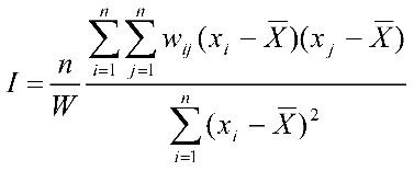
Here I is the Moran’s criterion,
n – the number of objects in space,
![]() – a mean value of an attribute,
– a mean value of an attribute,
![]() – values of an attribute for objects i and j,
– values of an attribute for objects i and j,
w – a spatial weight for a pair of objects,
W – the sum of spatial weights.
Let us explain the meaning of this formula. The calculation is done with several steps:
1) First, one needs to calculate a mean value of an attribute (![]() ).
).
2) The next step is to calculate for each object a difference between single value and a mean (![]() ).
).
3) The third step is to square each difference calculated at the previous step and to get a sum of these squares:

4) For each pair of objects spatial weights are defined (w). These weights show how big is a reciprocal influence between the objects. There are different ways to define the spatial weights. The most common way is to define them on the basis of a distance between the objects. In the simplest case, the weight is defined as an inverse distance, i.e. one divided by a distance.
5) Then, a sum of spatial weights is calculated (W):

6) The number of objects is divided by the sum of spatial weights:
![]()
7) Then, for each pair of objects differences between single values and a mean are multiplied one by another and by a spatial weight:

8) At the final step, the product obtained at the previous step is divided by the sum of quadrates obtained at the third step and multiplied by the sum of spatial weights obtained at the sixth step. Finally, we get the Moran’s I criterion value that is to be compared to its expected value.
The expected value of the Moran’s I criterion that should mark a random distribution of values is calculated as:

In this formula, E[I] is the expected value of the Moran’s criterion, n – the number of objects. According to this formula, the bigger is the number of objects the closer are values of E[I] to zero.
Comparing І to Е[I], one should make a decision about whether the difference between them is statistically significant. To do so the z-criterion is applied, however, its calculations are even more sophisticated than those we described above. So we omit them for now. Details on the calculations of z-criterion can be found here and here.
Practice
Let us describe manipulations with the Moran’s I criterion by means of the ArcGIS software using the following example. We took a vector layer with municipalities around the city of Belgorod (Russian Federation), approximating the Belgorod Metropolitan Area (fig. 2). Among the attributes of this layer, there is a field with the percentage of inhabitants who were born outside the Belgorod region. This information is taken from the base of the 2002 population census microdata. We need to define how these values are distributed.
When we are making visualisation of our spatial data we could assume on the character of their distribution. But such assumptions may not lead to correct conclusions due to their subjectivity. Moreover, the perception of cartographic visualisation may differ depending on the chosen grading and colour scales. Therefore, to make an objective evaluation the qualitative analytical approaches should be applied.
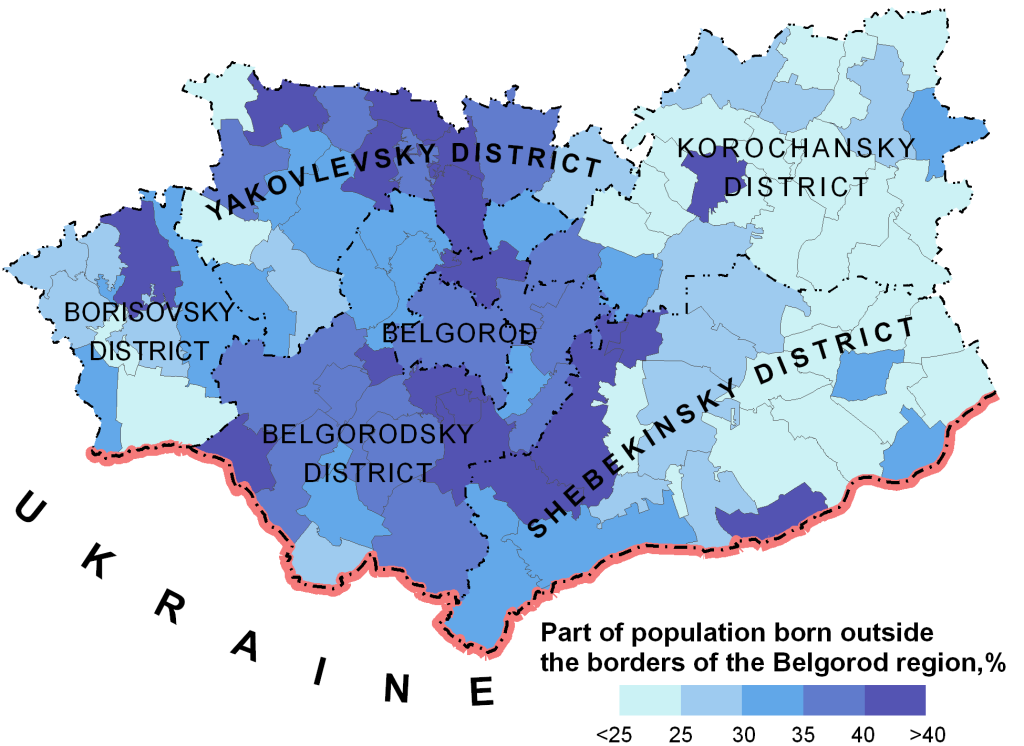
Fig. 2. The percentage of inhabitants who were born outside the Belgorod region (from top to down, left to right: Yakovlivka, Korocha, Borisovka, Belgorod, and Shebekine Districts)
1) To launch the calculation of the Moran’s I criterion select from the Toolbox (ArcToolbox) the command Spatial Statistic Tools → Analyzing Patterns → Spatial Autocorrelation (Moran’s I) (fig. 3). There appears the window Spatial Autocorrelation (Moran’s I), in which you should to adjust the procedure parameters (fig. 4).
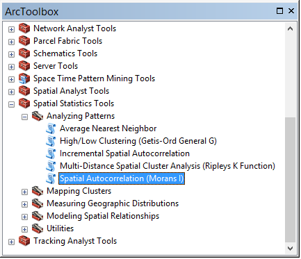
Fig. 3. The tool to calculate the Moran’s I criterion in the ArcToolbox
2) In the field Input Feature Class, identify the vector layer containing the data to be analysed.
3) In the list Input Field, specify the field (graph) from the Attribute Table for which the Moran’s I criterion should be calculated.
4) Check the option Display Output Graphically, in order to get the graphics report with calculation results.
5) From the list Conceptualization of Spatial Relationships select the way to conceptualise spatial relations. In other words, specify the way to calculate the spatial weights. This is an important parameter the calculation result depends on.
ArcGIS proposes to choose between the options:
Inverse Distance,
Inverse Distance Squared,
Fixed Distance Band,
Zone of Indifference,
Polygon Contiguity (First Order),
Get Spatial Weight From File.
To select the conceptualising option correctly one should know very well the studied area and phenomena. One should mind how one object influences another depending on the mode of reciprocal location and the distance between them.
Peculiarities of conceptualising spatial relations will be discussed in a separate post. By default, ArcGIS proposes the option Inverse Distance that will be used in our example.
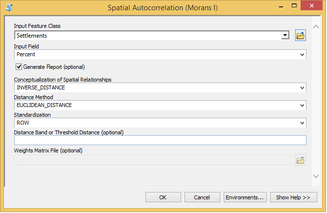
Fig. 4. The window for adjusting parameters to calculate the Moran’s I criterion
6) Select the distance measuring method in the field Distance Method. Here are two methods – the Euclidean and the Manhattan (City Block) Distance. The Euclidean distance is selected by default. We will use it in our example.
7) From the list, Standardization select an option for standardising the spatial weights. Here are two options proposed – None and Row. The None option is selected by default, that is standardising won’t be applied, and the absolute values of spatial weights will be used for calculations. If the Row option is selected each spatial weight value will be divided by the sum of spatial weights. Calculated in such a way, weight values will range from 0 to 1. Normalising is recommended when, – according to the option for calculating spatial weights, – different objects would have different numbers of neighbours.
8) Use the value from the row Distance Band or Threshold Distance (optional) for defining the number of neighbours to be used in the calculation of the Moran’s I criterion. This is a neighbour search radius. This value could be blank (by default), equal to 0 or be greater than 0. For each approach to conceptualise spatial relations these values influence the number of neighbours in their own ways. In our example, this value is taken by default.
If we use an inverse distance while calculating spatial weights, the blank value will allow the program to find such a distance that each object should have at least one neighbour. At zero, all existing objects will make neighbours to any single object. At the value greater than zero, only those objects matching the area outlined with a search radius will make neighbours.
9) When all calculation parameters are adjusted click the OK button in the window Spatial Autocorrelation (Moran’s I). We will get a graphic report as an html-file (fig. 5).

Fig. 5. Graphic report with the results of spatial autocorrelation assessment
Let us explain the obtained calculation result. For our data, we got the value of the Moran’s I criterion I = 0.47. For random distribution, the expected value of general Moran’s index is E[I] = -0.01. The probability of the first-type error (p-value) i.e. that our conclusion is wrong is less than 0.05. This means that the difference between calculated and expected values of the Moran’s criterion is statistically significant. Therefore, we obtained the positive spatial autocorrelation of the attribute. The per cent of people that were born outside the Belgorod region features the clustered (grouped) mode of distribution. Why it happened so is the topic of other research. We can say only that current picture reflects the difference in municipalities’ attractiveness for migrants. And to great extent, such a distribution has formed in the 1990s.


