Classification accuracy assessment. Confusion matrix method

Applying any classification algorithm to interpret a remotely sensed image we are always interested in the result accuracy. The simplest way to assess it is the visual evaluation. Comparing the image with the results of its interpretation, we can see errors and roughly estimate their size. But if we need a reliable accuracy assessment, we can’t do without quantitative methods of evaluation.

 

Theory

A confusion matrix (or error matrix) is usually used as the quantitative method of characterising image classification accuracy. It is a table that shows correspondence between the classification result and a reference image. I.e., to create the confusion matrix we need the ground truth data, such as cartographic information, results of manually digitizing an image, field work/ground survey results recorded with a GPS-receiver.

An illustration of the confusion matrix is shown in table 1. Let’s discuss its contents. Columns of table 1 are the ground truth classes, and rows of the table are the classes of the classified image to be assessed. Cells of the table show number of pixels for all the possible correlations between the ground truth and the classified image.

What sort of information can we get from the confusion matrix?

Firstly, we should pay attention to the diagonal elements of the matrix. In table 1, they are highlighted with blue. Diagonal cells contain the number of correctly identified pixels. If we divide the sum of these pixels by the total number of pixels we will get classification’s overall accuracy (OvAc). For the confusion matrix shown in table 1 this index will be equal to:

OvAc = ( aA + bB + cC ) / N = ( 37 + 25 + 43 ) / 142 ≈ 0,74

Another accuracy indicator is the kappa coefficient. It is a measure of how the classification results compare to values assigned by chance. It can take values from 0 to 1. If kappa coefficient equals to 0, there is no agreement between the classified image and the reference image. If kappa coefficient equals to 1, then the classified image and the ground truth image are totally identical. So, the higher the kappa coefficient, the more accurate the classification is.

Apart from the overall accuracy, the accuracy of class identification needs to be assessed. In order to do that, we have to look at non-diagonal cells in the matrix. These cells contain classification errors, i.e. cases when the reference image and the classified image don’t match. There are two types of errors: underestimation (omission errors, omission) and overestimation (commission errors, commission).

For any class, errors of commission occur when a classification procedure assigns pixels to a certain class that in fact don’t belong to it. Number of pixels mistakenly assigned to a class is found in column cells of the class above and below the main diagonal. For class A, commission errors are marked pale-yellow in table 1. The sum of these cell pixels is the absolute value of the class commission. And if we divide this sum by the total number of class pixels, we will get the relative commission error (Com):

Сom = ( bA + cA ) / ∑A = ( 9 + 11 ) / 57 ≈ 0,35

The amount of errors of commission is also described by the Producer’s accuracy (PrAc) indicator. It is the number of correctly identified pixels divided by the total number of pixels in the reference image. For class A in table 1:

PrAc = aA / ∑A = 37 / 57 ≈ 0,65

Com and PrAc values are connected:

PrAc = 1 – Сom

For any class, errors of omission occur when pixels that in fact belong to one class, are included into other classes. In the confusion matrix, the number of omitted pixels is found in the row cells to the left and to the right from the main diagonal. For class A, omission errors are marked in orange. The sum of these cells is the absolute value of the class omission. And if we divide this sum by the total number of class pixels in the classified image, we will get the relative omission error (Om):

Om = ( aB + aC ) / ∑a = ( 3 + 7 ) / 47 ≈ 0,21

User’s accuracy (UsAc) is another index characterising the amount of errors of omission. It is the number of the correctly identified pixels of a class, divided by the total number of pixels of the class in the classified image. For class A in table 1 it equals:

UsAc = aA / ∑a = 37 / 47 ≈ 0,79

Om and UsAc values are connected:

UsAc = 1 – Om

As you can see, there are several classification accuracy indicators. Thus a question arises: what indicators should be provided to correctly describe the accuracy? At least the overall accuracy of classification or kappa coefficient should be indicated. But it will be an incomplete description. It is better to include the values of commission and omission errors. As the overall accuracy itself can be misleading. It is possible that the overall accuracy might be quite high, whereas an individual class or several classes will contain a considerable amount of errors. And if the accuracy of those very classes is the most important to a user, the classification results cannot be acceptable despite their high overall accuracy. Additionally, the producer’s and user’s accuracy values cannot be separately used as an indication of the classification accuracy, as these values do not show a complete picture.

 

Practice

Now we will see how to calculate and interpret the confusion matrix in ENVI software. Confusion Matrix tool enables us to do that. It creates the confusion matrix and error images for each class. In addition it calculates the classification accuracy assessment indices (overall accuracy, kappa coefficient, omission and commission errors for each class).

In figure 1, on the left, is a fragment of Landsat 5 TM image taken on 16.09.2009. It covers the territory of Siverskiy Donets’ floodplain to the south of Mokhnach, Zmiiv district, Kharkiv region, Ukraine. Band combination of 4:5:3 was used to display this image. In this combination, vegetation is orange (deciduous forests) and brown (coniferous forests). Emerald-green is soil (darker shades) and dry grass (lighter shades). Water bodies are dark-blue.

The image was classified distinguishing three classes: deciduous forests, coniferous forests and water bodies (fig.1, centre). There is a fourth class as well – unclassified pixels, i.e. everything that can’t be attributed to the other three classes. On the right in figure 1 is a  reference image created from digitizing manually. We will use it to calculate the confusion matrix.

Fig. 1. Left to right: fragment of the Landsat image, classified image, reference image

 

Creating the confusion matrix

1) To create the confusion matrix, go to Classification → Post Classification → Confusion Matrix Using Ground Truth Image.

2) A pop-up will appear where you have to select a classified image for which accuracy is assessed. Choose the image and press OK.

3) In the next pop-up, select the  reference image. Press OK.

4) After both images are selected, correspondence between specific classes of the classified image and the ground truth image has to be assigned. This operation must be completed in the Match Classes Parameters dialog. Match the classes of the ground truth image and the classified image into pairs for comparison. To do so, select both classes and click the Add Combination button.

Fig. 2. Matching classes of the classified image and ground truth

 

5) After matching classes into pairs for comparison, a pop-up will appear where parameters of the confusion matrix must be set. This pop-up contains three parameter groups listed from top-down:

– output units for cells of the confusion matrix (Output Confusion Matrix in)

– accuracy report creation (Report Accuracy Assessment)

– error images creation (Output Error Images)

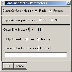
Fig. 3. Setting parameters of the confusion matrix

Output values for the confusion matrix can be pixels or percents. To choose the first option, check Pixels next to Output Confusion Matrix in. To choose the second option, check Percents. Also, two confusion matrices can be created simultaneously – one with values in pixels, and another one – in percents. To do that, check both options.

If you wish to see the report on classification accuracy, toggle Yes next to Report Accuracy Assessment. Otherwise toggle No.

To see which pixels were classified correctly and which were classified mistakenly, set the Output Error Images option to Yes.

After setting all parameters, press OK and finally, the calculated confusion matrix will appear in the Class Confusion Matrix window (fig. 4).

 

Analysing the confusion matrix

Let’s see what is displayed top-down in the Class Confusion Matrix window (fig. 4).

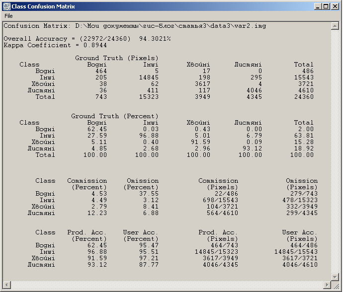
Fig. 4. Confusion matrix

The first row has a file path of the classified image which the accuracy assessment is performed for. Next are the overall accuracy and kappa coefficient. Below is the confusion matrix itself. First, in pixel values, and then – in percent values. Below the confusion matrix is the accuracy assessment report: commission and omission values for each class.

The overall classification accuracy for the image provided in figure 1 equals nearly 94%. E.g. about 94% of pixels are correctly assigned, and 6% of pixels are assigned with errors. This is quite a high accuracy.

Also, each specific class accuracy is shown in the matrix. From the three classes, deciduous forests have the highest classification accuracy (93.12%), next are coniferous forests (91.59%), and water bodies have the lowest classification accuracy (62.45%). The first two classes’ accuracy can be considered high, it is hardly so for the third class.

Next we will analyze the size of commission and omission errors for each class. We can see that omission errors are more common for water bodies and coniferous forests. And on the contrary, for deciduous forests, commission errors prevail.

It depends on the goal and strategy of interpretation to decide on the better balance of commission and omission. In some cases identification of all pixels actually belonging to a certain class may be essential – even with the increase in the number of upward distortions. In other cases it is better to have gaps than to include into a class pixels that do not belong to it. Usually the users don’t choose these marginal options, but seek a compromise between them.

Analysing output error images

Classification error image is a multi-layer raster image. Every layer corresponds to a separate class. In ENVI, error images show only omission errors. Every layer has only two pixel values – 0 and 1. The first value is a correctly identified pixels, and the second value is an omitted pixels.

It is more convenient to analyse the error image when it is overlaid onto the reference image and set half-transparent. We need to perform the following steps to do  that.

1) In the table of contents (Layer Manager) drag the error image layer up so that it appears above the reference image layer (fig. 5).

2) Toggle off all the classes of the reference image apart from the one which we visualise the classification errors for.

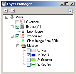
Fig. 5. Error image and reference image in the Layer Manager

3) Right-click the layer name. In the context menu select Change RGB Bands… A pop-up will appear where you can specify the layer with the error image (fig. 6).

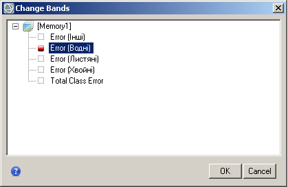
Fig. 6. Choosing a layer to display

4) Dragging the Transparency slider, set the transparency value for error image from 0 to, say, 40 (fig. 7).

Fig. 7. Transparency slider

Visualisation of errors for each of the three classes is shown in figure 8. Looking at these images, we can make certain conclusions about spatial patterns of errors. So, in this example, omission errors have primarily occurred on the boundaries of the identified objects. Large objects were classified better than small objects, i.e. small objects have a higher proportion of errors in the total area. At the same time, small objects of equal area have different portions of errors. Compact objects were identified better than stretched objects.

Fig. 8. Error images (water bodies, deciduous forests, coniferous forests)

 

To conclude, let’s once again get back to the goal of creating the confusion matrix. As I mentioned in the beginning, the matrix is calculated to assess the classification accuracy. That is true, but that is not all. Analysis of the confusion matrix and error images helps us to reveal the sources of errors, and based on that, we can look for ways to improve the classification accuracy.