While performing supervised classification it is possible to obtain, in addition to the classified map, the rule images of your classification. You can learn what they are, and how to view these images can in a previous post. This post is about how to improve the quality of the classification with the help of rule images. That is, it will be about so-called “rule-based classification”. This is not an independent method of classification, but rather an addition to other methods. It is used in complex cases of processing to facilitate the selection of optimal threshold values for the criterion used for determination of classes.
With regard to the very term put into the name of this post, it is necessary to give an important warning. “Rule-based classification” can also refer to object-based analysis. This should be borne in mind when searching for literature on the topic.
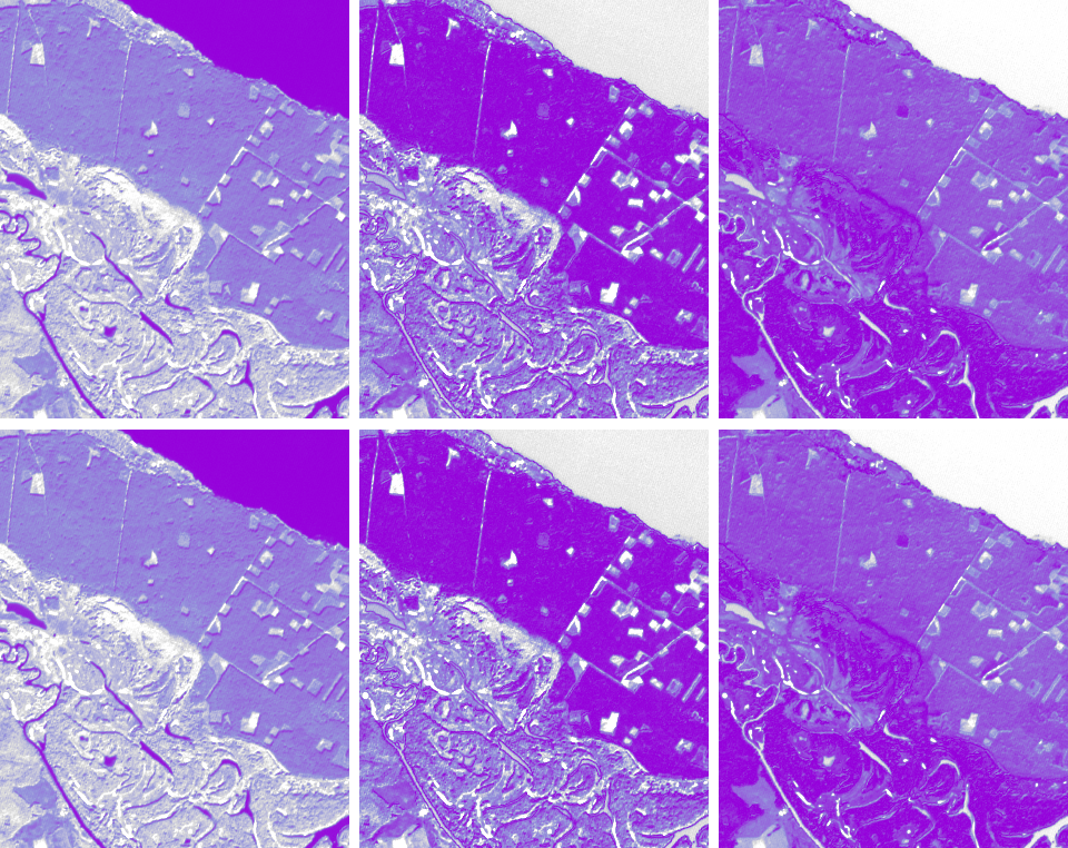
We will look into the practical application of the rule-based classification in an example, which previously illustrated the minimum distance algorithm. In this example, three classes were derived from ASTER VNIR: water bodies, coniferous forests and deciduous forests (Fig. 1).

Fig. 1. Satellite image and rule images for water bodies, coniferous and deciduous forests (from left to right)
1) To work with image rules, you first need to create them, and for this purpose – to execute a supervised classification by any algorithm. That is why the classification from the rule images is categorized as the post-classification processing of images.
2) When we already have the rule image, then you can start a classification based on them. To do this, select the Classification → Post Classification → Rule Classifier in the ENVI Toolbox.
3) A window will appear in which you need to select a rule image. Select it and click OK in this window.
4) After selecting the rule image, the Rule Image Classifier Tool window will appear (Figure 2). Let’s look at the window contents.

Fig. 2. Rule Image Classifier Tool
In the Rule Image Classifier Tool there are three main classification settings:
– classification mode (Classify by),
– a list of classes,
– a threshold value (Thresh:).
5) Classify by (classification mode) is how we determine the pixel belonging to the class according to the mathematical classification criterion. There are two options. The first option is when the class obtains pixels with classification values smaller than the threshold (classification by the minimum value, Minimum Value). In the second option, on the contrary, the class obtains pixels with classification values greater than the threshold (classification by the maximum value, Maximum Value).
To specify a classification mode, you need to press the switch button. In our case, the correct option is the classification by the minimum value, since the rule image is for the minimum distance algorithm classification. And in this algorithm, a pixel is assigned to the class with the center closest to this pixel.
A comparison of the two modes of classification for our example is shown in Figure 3. We see that when classifying the minimum values for a class of water bodies, in fact, they are correctly classified (fig. 3, right). And when classifying for the maximum value, all types of water bodies are not classified as such (fig. 3, left).

Fig. 3. Comparison of the classification to the maximum (left) and the minimum (right) value. In the center – the rule image of the classification for reservoirs
6) The list of classes contains their names and colors. In our example (Fig. 2) we have three classes under the names water, conifer, deciduous. They are respectively blue, dark green and light green. Next to each color in the class, on the left, in the Rule Image Classifier Tool, there are class switches. If you uncheck them, then the corresponding class will not be allocated during the classification. By default, all available classes are enabled. The number of these classes is equal to the number of layers in the classification image.
7) The next step is to enter a threshold value. To give all classes the same value, type it in the input line next to the Set All Threshold button. And then click it. To set different thresholds for each class, enter them in separate input lines (Thresh:), which are to the right of the list of classes.
8) For an easier selection of the threshold value, the Rule Image Classifier Tool window provides two tools: creating histograms and calculating descriptive statistics from the rule image. Both tools allow you to see what values are in the rule image for a particular class and how they are distributed.
To create a histogram, you need to click on one of the Hist buttons to the right of the input lines (Thresh:). A window with a histogram will appear. Figure 4 shows a window with a histogram of the mathematical criterion (distance to the center of the class) for reservoirs. We see a few peaks on it. Each peak corresponds to some class of objects or a group of classes. The most interesting is one of the two extreme peaks (on the sides). If we make a classification for a minimal value, then we must pay attention to the leftmost peak – the peak at the smallest values (just our case). Somewhere between it and the next peak on the X-axis (Data Value in Fig. 4) is the optimal threshold. And if we make the classification by the maximum value, then, on the contrary, we need to look at the extreme right peak at the highest values. Analyzing the histogram for reservoirs (Figure 4), it can be argued that the optimal threshold is somewhere between five and 20.

Fig. 4. Distances to the center of the class histogram for water bodies
9) To view statistics for the rule image, select Options → Stats for Selected Rule Bands from the Rule Image Classifier Tool. The Statistics Results window appears (Figure 5). The bottom of this window lists the quantitative values for each rule image layer: minimum, average, maximum, and standard deviation from the average. There is also information on the frequency of each available value – the number of pixels with that value and the percentage of such pixels from the total image size.
Statistics are accompanied by graphs that are located at the top of the Statistics Results window. There are several variations that are selected from the drop-down list when you click the Select Plot button. The most informative graphs are histograms of all layers of the classification rule image (Fig. 5, left) and the graph of change between layers of this image of minimum, maximum and average values (Fig. 5, right).

Fig. 5. Statistics Results window with descriptive statistics and statistical graphs
10) When all the settings are complete, click the Quick Apply button. Then a window will appear to preview the result. If you like it, click the Save To File … button to save the result. If you do not like it, choose other threshold value. In the end, by trial and error, you will find the optimal combination of thresholds.
Figure 6 shows the classification results obtained for different threshold values. Figure 6A is the result of the same for all and low threshold values. For each class, the threshold is equal to three. This is too small. Therefore, numerous errors of omission occurred. Each class is less than its actual area. Deciduous forests suffered the most, and water was affected least by this.
Figure 6B is the result of the same for all and overestimated threshold values. For each class, the value of the criterion is 30. This value is too high. Therefore, numerous errors of commission occurred. The class of coniferous forests was erroneously attributed to the share of non-forested areas and deciduous forests. In turn, the deciduous forests are incorrectly attributed to the grassy vegetation of the floodplain. Only reservoirs are separated precisely.
Figure 6C is the result of different but incorrectly balanced threshold values. The area of deciduous forests is bigger than in reality, and the area of reservoirs and coniferous forests is less than in reality.
Figure 6D is the result of different and optimally balanced threshold values.

Fig. 6. Results of classifications obtained with different combinations of threshold values
The use of classification rule images is not limited to selecting the optimal combinations for the thresholds for which the classes are depicted in the illustrations. Another direction of their use is the analysis of the accuracy of classification by the method of ROC-curves (ROC-analysis). A separate post will be dedicated to this topic.


